Given an appropriate network architecture, gradient-based learning algorithms can be used to synthesize a complex decision surface that can classify high-dimensional patterns, such as handwritten characters, with minimal preprocessing.
Gradient descent is an optimization algorithm used to minimize some function by iteratively moving in the direction of steepest descent as defined by the negative of the gradient. In machine learning, we use gradient descent to update the parameters of our model.
To calculate the gradient of a straight line we choose two points on the line itself. From these two points we calculate: The difference in height (y co-ordinates) ÷ The difference in width (x co-ordinates). If the answer is a positive value then the line is uphill in direction.
The steepness of the slope at that point is given by the magnitude of the gradient vector. The gradient can also be used to measure how a scalar field changes in other directions, rather than just the direction of greatest change, by taking a dot product. Suppose that the steepest slope on a hill is 40%.
A simple gradient Descent Algorithm is as follows:
- Obtain a function to minimize F(x)
- Initialize a value x from which to start the descent or optimization from.
- Specify a learning rate that will determine how much of a step to descend by or how quickly you converge to the minimum value.
Gradient descent is an optimization algorithm that finds the optimal weights (a,b) that reduces prediction error. Step 2: Calculate the gradient i.e. change in SSE when the weights (a & b) are changed by a very small value from their original randomly initialized value.
Selecting a learning rateNotice that for a small alpha like 0.01, the cost function decreases slowly, which means slow convergence during gradient descent. Also, notice that while alpha=1.3 is the largest learning rate, alpha=1.0 has a faster convergence.
It gives us the global minimum, since the cost function is bell shape. For large n calculating the summation in gradient descent is computationally expensive. We called this type as batch gradient descent, since we are looking at all training set at a time.
Gradient boosting is a type of machine learning boosting. It relies on the intuition that the best possible next model, when combined with previous models, minimizes the overall prediction error. If a small change in the prediction for a case causes no change in error, then next target outcome of the case is zero.
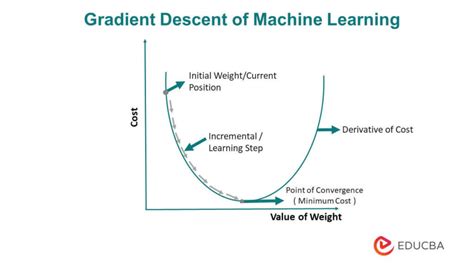
Gradient Descent is the process of minimizing a function by following the gradients of the cost function. This involves knowing the form of the cost as well as the derivative so that from a given point you know the gradient and can move in that direction, e.g. downhill towards the minimum value.
Momentum, simply put, adds a fraction of the past weight update to the current weight update. This helps prevent the model from getting stuck in local minima, as even if the current gradient is 0, the past one most likely was not, so it will as easily get stuck.
Adam [1] is an adaptive learning rate optimization algorithm that's been designed specifically for training deep neural networks. The algorithms leverages the power of adaptive learning rates methods to find individual learning rates for each parameter.
Batch Gradient DescentIt is a greedy approach where we have to sum over all examples for each update.
CPU and GPU memory architecture usually organizes the memory in power of 2. (check page size in your CPU by getconf PAGESIZE in Linux) For efficiency reason it is good idea to have mini-batch sizes power of 2, as they will be aligned to page boundary. This can speed up the fetch of data to memory.
Gradient descent is also known as steepest descent, or the method of steepest descent. So, there's no difference.
Well, a cost function is something we want to minimize. For example, our cost function might be the sum of squared errors over the training set. Gradient descent is a method for finding the minimum of a function of multiple variables. So we can use gradient descent as a tool to minimize our cost function.
This simple, effective, and widely used approach to training neural networks is called early stopping. In this post, you will discover that stopping the training of a neural network early before it has overfit the training dataset can reduce overfitting and improve the generalization of deep neural networks.
Batch gradient descent is a variation of the gradient descent algorithm that calculates the error for each example in the training dataset, but only updates the model after all training examples have been evaluated. One cycle through the entire training dataset is called a training epoch.
The Gradient (also called Slope) of a straight line shows how steep a straight line is.
In general, batch size of 32 is a good starting point, and you should also try with 64, 128, and 256. Other values (lower or higher) may be fine for some data sets, but the given range is generally the best to start experimenting with.
Also, on massive datasets, stochastic gradient descent can converges faster because it performs updates more frequently. Also, the stochastic nature of online/minibatch training takes advantage of vectorised operations and processes the mini-batch all at once instead of training on single data points.
The key practical problems are: converging to a local minimum can be quite slow. if there are multiple local minima, then there is no guarantee that the procedure will find the global minimum (Notice: The gradient descent algorithm can work with other error definitions and will not have a global minimum.
According to gradient descent rule, we should update the weight according to w = w - df/dw.
To summarize: in order to use gradient descent to learn the model coefficients, we simply update the weights w by taking a step into the opposite direction of the gradient for each pass over the training set – that's basically it.